本文由 AI(Trae Agent) 检索、整理并撰写,尚未经过人工逐条校对。所有数字来自随文附带的 R 脚本(scripts/00_data.R 至 06_synthesis.R)的真实运行结果,图由这些脚本生成。四套真实数据分别是 airway(RNA-seq)、NormalyzerDE 的 LFQ 稀释系列、10x PBMC 3k 与 CLL/sacurine;模拟实验的生成参数与真值都写在代码里。方法实现以公开公式为准,并与 edgeR、DESeq2、limma、vsn 的官方结果做过抽查;两者不完全一致的地方在正文注明。
This article was researched and written by an AI system (Trae Agent) and has not been proofread line by line by a human. Every number comes from an actual run of the R scripts shipped with the post (scripts/00_data.R … 06_synthesis.R), and every figure is produced by those scripts. The four real datasets are airway (RNA-seq), the NormalyzerDE LFQ dilution series, 10x PBMC 3k, and CLL/sacurine; all simulation parameters and ground truth are in the code. Implementations follow the published formulas and were spot-checked against edgeR, DESeq2, limma and vsn; any disagreement is stated in the text.
写一篇中英双语长文,系统比较 R 里用于转录组与蛋白质组的归一化方法。要求:讲清每种方法的数学公式、算法步骤、R 实现与失效条件;用真实数据展示归一化前后的分布、PCA、相关性、下游差异;用模拟数据(已知真值)量化偏差、RMSE、FDR/TPR;覆盖 bulk RNA-seq、LFQ 蛋白组、单细胞、芯片与代谢组;所有方法先自实现再与官方包对照;正面与负面结果都如实报告。
A long bilingual comparison of normalisation methods used in R for transcriptomics and proteomics. Cover the formula, algorithm, R implementation and failure mode of each method; use real data to show distributions, PCA, correlations and downstream differential expression; use simulations with known truth to quantify bias, RMSE, FDR and TPR; span bulk RNA-seq, LFQ proteomics, single-cell, microarray and metabolomics; implement each method from its formula and cross-check the official package; report positive and negative results honestly.
1. 七种归一化,同一批数据 / Seven normalisations, one dataset
先把结论摆在桌面上。下面是 airway 的 8 个样本、63,677 个基因,用七种常见方法归一化后的分布:CPM、TPM、上四分位(UQ)、median-of-ratios(MoR)、RLE、TMM、quantile(QN),最后加一个 VST。它们看起来都很”整齐”,但整齐的方式不同:有的把中位数对齐,有的把整个分布对齐,有的只对齐一个分位数。
Put the conclusion on the table first. Below are 8 airway samples and 63,677 genes after seven common normalisations: CPM, TPM, upper quartile (UQ), median-of-ratios (MoR), RLE, TMM and quantile (QN), plus VST. They all look “tidy”, but in different ways: some align medians, some align the whole distribution, some align a single quantile.
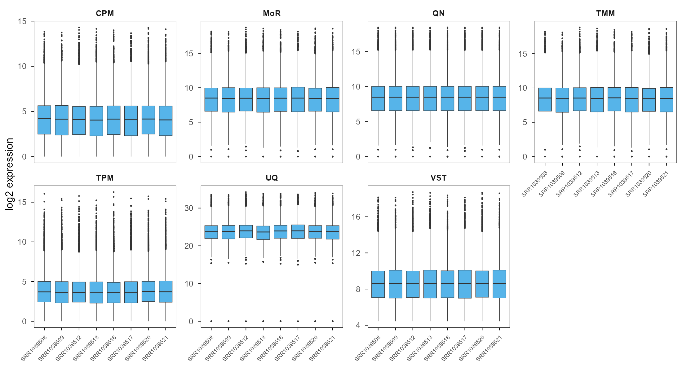
这张图最容易被误读成”方法之间差别不大”。真正的问题是:它们各自把什么当成技术噪声,又把什么当成生物信号? 如果一批数据里 40% 的基因都上调,TMM 与 RLE 会认为”多数不变”这个前提失效;如果所有基因都上调 2 倍,没有任何基于组成的归一化能看见它。归一化的差别不在分布好不好看,而在这些前提被违反时会发生什么。
The easy misreading is “the methods hardly differ”. The real question is: what does each method treat as technical noise, and what as biological signal? If 40% of genes go up, TMM and RLE lose their “most genes are unchanged” premise; if every gene doubles, no composition-based method can see it. The difference between methods is not how tidy the boxes look, but what happens when those premises fail.
2. 归一化是守恒量的声明 / Normalisation is a claim about an invariant
我把归一化定义为一个声明:在样本 \(j\) 上乘以或除以一个因子 \(s_j\),使得某个统计量在样本之间保持不变。不同的 \(s_j\) 就是不同的守恒量。总量法声明”每个样本的总 RNA/总蛋白相同”;参照比值法声明”多数特征不变”;分布匹配法声明”每个样本的分布形状相同”;方差稳定法声明”均值与方差的关系已知”;spike-in 法声明”外源锚点的量已知”。
A normalisation is a claim: multiply or divide sample \(j\) by a factor \(s_j\) so that some statistic stays constant across samples. Different \(s_j\) mean different invariants. Total-count methods claim “each sample has the same total RNA/protein”; reference-ratio methods claim “most features are unchanged”; distribution-matching methods claim “each sample has the same distribution shape”; variance-stabilising methods claim “the mean–variance relation is known”; spike-in methods claim “the amount of an external anchor is known”.
| 家族 / Family | 守恒量 / Invariant | 代表 / Examples | 何时失效 / Fails when |
|---|---|---|---|
| 总量 / total | 每样本总量 / total per sample | CPM、TPM、TIC、iBAQ | 全局上调、组成变化 / global shift, composition |
| 参照比值 / ratio | 多数特征不变 / most unchanged | RLE、MoR、TMM、MaxLFQ | 多数差异、大量缺失 / many DE, many missing |
| 分布匹配 / distribution | 分布形状相同 / same shape | quantile、loess、UQ | 真实分布不同 / real distribution differs |
| 方差稳定 / variance | 均值–方差关系 / mean–variance law | VSN、VST、rlog | 关系估错、零膨胀 / wrong law, zero inflation |
| 外部锚点 / anchor | spike-in 量已知 / known spike | ERCC、UPS1 | 锚点丢失 / anchor lost |
| 批次模型 / batch | 批次是可加/可乘 / additive or multiplicative | ComBat | 与条件混杂 / confounded with condition |
English: one row per family; the third column names representative methods and the fourth the condition under which the invariant fails.
后面每一节都会回到这张表。读公式时先问”它在估哪个 \(s_j\)“,读实验时先问”这个场景违反了哪一行”。
Every later section returns to this table. When reading a formula, ask “which \(s_j\) is it estimating”; when reading an experiment, ask “which row does this scenario violate”.
3. 基础概念:组成数据与相对丰度 / Compositional data
RNA-seq 与质谱给出的都不是绝对量,而是相对丰度:一个基因的读数取决于它占文库的比例,一个肽的强度取决于它占离子流总量的比例。这类数据叫组成数据(compositional data)。它的麻烦在于:所有分量被约束在一个总和上,一个分量上升,其他分量必然被压低,即使它们的绝对量没变。
RNA-seq and mass spectrometry do not measure absolute amounts but relative abundances: a gene’s read count depends on its share of the library, a peptide’s intensity on its share of the total ion current. Such data are compositional. The trouble is that all parts are constrained to a sum: when one part rises, the others are pushed down even if their absolute amounts did not change.
这解释了一个反直觉的现象:如果所有基因同时上调 2 倍,CPM、TPM、UQ、MoR、RLE、TMM、QN 都会估计出”没有变化”。 因为它们的输入只有比例,比例里没有”总量”这一维。只有 spike-in 或已知的外参能打破这个约束。
This explains a counter-intuitive phenomenon: if every gene doubles, CPM, TPM, UQ, MoR, RLE, TMM and QN all estimate “no change”. Their input is proportions, and proportions have no “total” axis. Only spike-ins or an external reference can break the constraint.
处理组成数据有一套专门的语言:CLR(centered log-ratio)把每个分量除以几何均值再取对数,\(\mathrm{clr}(x)_i=\log x_i-\frac{1}{D}\sum_j\log x_j\);ILR further 用正交基把 \(D\) 维压缩到 \(D-1\) 维。它们不估计 \(s_j\),而是把”相对”这件事直接写进坐标。代价是零值需要伪计数,且结果的解释不再是”表达量”。
Compositional data have their own language: CLR (centred log-ratio) divides each part by the geometric mean and takes logs, \(\mathrm{clr}(x)_i=\log x_i-\frac{1}{D}\sum_j\log x_j\); ILR goes further and uses an orthonormal basis to reduce \(D\) parts to \(D-1\) coordinates. They do not estimate \(s_j\); they build relativity into the coordinates. The price is a pseudocount for zeros and an interpretation that is no longer “expression level”.
4. 基础概念:计数、强度与缺失 / Counts, intensities and missing values
转录组与蛋白质组的噪声结构不同。RNA-seq 的计数近似负二项:方差随均值上升,低表达基因的相对噪声更大,零很多但通常是”没测到”而不是”不存在”。LFQ 质谱的强度近似对数正态,低丰度蛋白更容易缺失,而且缺失往往是 MNAR(missing not at random)——缺失本身携带”丰度低”的信息。
Transcriptomics and proteomics have different noise structures. RNA-seq counts are approximately negative binomial: variance grows with the mean, low-expression genes are relatively noisier, and zeros are usually “not observed” rather than “absent”. LFQ intensities are approximately log-normal; low-abundance proteins go missing more often, and the missingness is usually MNAR (missing not at random) — the missingness itself carries the information “low abundance”.
这个差别决定了归一化的顺序。计数数据可以先归一化再取 log,因为零的分布相对简单;蛋白组如果先把缺失当零,低丰度蛋白会被系统性地压低,之后无论怎么归一化都救不回来。本文第 29 节会看到:先过滤到完整蛋白,保留 23% 的特征但保住了功效;先做最小区间插补,保留 100% 的特征却把 TPR 打到 0。
This difference dictates the order of operations. Counts can be normalised and then logged because zeros are comparatively simple; in proteomics, treating missing values as zero systematically pushes low-abundance proteins down, and no later normalisation can undo it. Section 29 shows the trade-off: filtering to complete proteins keeps 23% of features but preserves power; minimum imputation keeps 100% of features and drives TPR to 0.
5. 基础概念:log 与方差稳定 / Logs and variance stabilisation
取 log 是最常见的一步,但它不是”让数据正态”的魔法。对于计数,\(\log(x+1)\) 在低计数处会引入压缩偏倚;对于强度,\(\log_2\) 把乘性误差变成加性误差,这是它有用的原因。方差稳定(variance stabilisation)是更进一步:找一个变换 \(h\),使 \(\mathrm{Var}(h(X))\) 近似与 \(\mathbb{E}[X]\) 无关。
Taking logs is the most common step, but it is not a magic “make it normal” button. For counts, \(\log(x+1)\) introduces compression bias at low counts; for intensities, \(\log_2\) turns multiplicative error into additive error, which is why it helps. Variance stabilisation goes further: find a transform \(h\) such that \(\mathrm{Var}(h(X))\) is approximately independent of \(\mathbb{E}[X]\).
负二项计数在参数化下有解析的稳定变换,DESeq2 的 VST 与 rlog 就是用数据估计离散度后再变换;质谱的 VSN 用 \(\operatorname{asinh}(a+bx)+c\),其中 \(a,b,c\) 由最大似然估计。它们与”先归一化再 log”的区别是:方差稳定把均值–方差关系也当成模型的一部分,因此对低丰度特征的处理更平滑。
Negative-binomial counts admit analytic stabilising transforms; DESeq2’s VST and rlog estimate dispersions and then transform, while mass-spectrometry VSN uses \(\operatorname{asinh}(a+bx)+c\) with \(a,b,c\) fitted by maximum likelihood. The difference from “normalise then log” is that variance stabilisation treats the mean–variance relation as part of the model, so low-abundance features are handled more smoothly.
6. 用什么评价归一化 / How to judge a normalisation
归一化没有”唯一正确”的输出,只有”在某个目标下更好”。本文用六个指标,分成两类。有真值时:log2 fold change 的偏差与 RMSE、BH 5% 下的 TPR 与 FDR。没有真值时:样本间相关性、组内标准差、聚类 ARI、以及主成分与已知协变量(批次、深度、条件)的关联。
There is no single correct output of normalisation, only “better for a stated goal”. Six metrics are used here, in two groups. With ground truth: bias and RMSE of log2 fold changes, TPR and FDR at BH 5%. Without ground truth: between-sample correlation, within-group standard deviation, clustering ARI, and the association of principal components with known covariates (batch, depth, condition).
这些指标不能互相替代。一个方法可以把 RMSE 压低,同时把 TPR 打到 0——第 29 节的插补就是例子;一个方法可以把样本相关性做到 0.99,同时把真实差异抹平——第 27 节的全局位移就是例子。每次只报一个数,几乎总能得到想要的结论。
These metrics are not interchangeable. A method can lower RMSE while driving TPR to 0 — the imputation in Section 29; another can push sample correlation to 0.99 while erasing real differences — the global shift in Section 27. Report one number and you can almost always get the conclusion you want.
7. 总量法:CPM、TPM、RPKM/FPKM / Total-count methods
CPM 最简单:把每个样本除以它的文库大小,再乘 \(10^6\),
CPM is the simplest: divide each sample by its library size and multiply by \(10^6\),
\[ \mathrm{CPM}_{ij}=\frac{c_{ij}}{\sum_{i'}c_{i'j}}\times 10^6 . \]
它只校正深度,不校正基因长度。RPKM/FPKM 先除以基因长度 \(\ell_i\),再除以文库大小;TPM 调换了顺序:先除以长度,再让每个样本的和为 \(10^6\),
It corrects depth only, not gene length. RPKM/FPKM divide by gene length \(\ell_i\) and then by library size; TPM swaps the order: divide by length first, then rescale each sample to sum to \(10^6\),
\[ \mathrm{TPM}_{ij}= \frac{c_{ij}/\ell_i}{\sum_{i'}c_{i'j}/\ell_{i'}}\times 10^6 . \]
TPM 与 RPKM 的差别不是”谁更正确”,而是归一化后的总量含义不同:TPM 的每列和恒为 \(10^6\),RPKM 不是。做样本间比较时,这个差别会影响”总量”这个守恒量的定义。三个方法都假设”总量相同”,因此在组成变化时会一起偏。
The difference between TPM and RPKM is not “which is more correct” but what the normalised total means: a TPM column always sums to \(10^6\), an RPKM column does not. For between-sample comparison this changes what “total” is held constant. All three assume “equal total”, so they fail together under composition shifts.
8. 上四分位与中位数强度 / Upper quartile and median intensity
上四分位(UQ)把每个样本除以它的第 75 百分位数(通常只算非零值),
Upper quartile (UQ) divides each sample by its 75th percentile (usually over non-zero values),
\[ s_j=Q_{0.75}\big(\{x_{ij}:x_{ij}>0\}\big). \]
它假设”高表达部分的尺度在样本间相同”,比总量法更稳健,因为少数极高表达的基因不会主导分母。蛋白组里对应的做法是中位数强度归一化:先取 log2,再减去每个样本的中位数。两者都只对齐一个位置,不改变分布形状。
It assumes “the upper part of the distribution has the same scale across samples”, which is more robust than total counts because a few extremely high features cannot dominate the denominator. The proteomics counterpart is median intensity normalisation: take log2 and subtract each sample’s median. Both align one location and leave the shape alone.
第 26 节的深度实验里,UQ 的 RMSE 是 0.484,比 CPM 的 0.443 高;原因是低计数基因的 75 分位数估计很不稳定,深度差一大,UQ 的因子就抖。稳健的统计量不一定给出稳健的因子,这是它在稀疏数据上的软肋。
In the depth experiment of Section 26, UQ has RMSE 0.484 versus 0.443 for CPM; the 75th percentile is unstable when many counts are small, so the factor jitters with depth. A robust statistic does not guarantee a robust factor — that is its weakness on sparse data.
9. RLE 与 median-of-ratios / RLE and median-of-ratios
RLE 与 DESeq2 的 median-of-ratios 是同一个思想的两副面孔:先为每个基因算一个跨样本的参照,再看每个样本相对参照偏移多少,最后取中位数。
RLE and DESeq2’s median-of-ratios are two faces of one idea: build a cross-sample reference for each gene, measure how far each sample deviates from it, and take the median.
\[ g_i=\Big(\prod_{j=1}^{m}c_{ij}\Big)^{1/m}, \qquad s_j=\operatorname{median}_i\frac{c_{ij}}{g_i}. \]
RLE 在 log 空间做同样的事:\(s_j=\exp\big(\operatorname{median}_i(\log c_{ij}-\overline{\log c_{i\cdot}})\big)\)。两者都假设多数基因不变;当中位数被大量差异基因占据时,因子会被拉向”没有差异”,把真实信号一起压掉。
RLE does the same in log space: \(s_j=\exp\big(\operatorname{median}_i(\log c_{ij}-\overline{\log c_{i\cdot}})\big)\). Both assume most genes are unchanged; when the median is occupied by differentially expressed genes, the factor is pulled toward “no difference” and suppresses the signal.
一个实现细节值得单独说:RLE 的因子是相对于文库大小的,真正的有效文库是 \(\text{lib}_j\times s_j\);只除以 \(s_j\) 而不乘文库大小,会把深度留在数据里。本文最初的实现就犯了这个错,图 1 与第 26 节的数字都是修正后的版本。这类错误不会报错,只会让结果”看起来还行但差一点”。
One implementation detail deserves its own paragraph: RLE factors are relative to library size, so the effective library is \(\text{lib}_j\times s_j\); dividing by \(s_j\) alone leaves depth in the data. The first implementation here made exactly this mistake, and Figure 1 and Section 26 use the corrected version. Such bugs do not throw errors; they just make the result “look plausible but slightly off”.
10. TMM:修剪均值 of M / TMM: trimmed mean of M values
TMM 选择一个参照样本 \(r\),对每个基因算 log 比值 \(M\) 与平均丰度 \(A\),
TMM picks a reference sample \(r\), computes a log ratio \(M\) and an average abundance \(A\) for each gene,
\[ M_{ij}=\log_2\frac{c_{ij}/N_j}{c_{ir}/N_r}, \qquad A_{ij}=\frac12\log_2\Big(\frac{c_{ij}}{N_j}\cdot\frac{c_{ir}}{N_r}\Big), \]
其中 \(N_j=\sum_i c_{ij}\)。然后按 \(M\) 的两端各去掉 30%、按 \(A\) 的两端各去掉 5%,用权重
where \(N_j=\sum_i c_{ij}\). It then trims 30% from each tail of \(M\) and 5% from each tail of \(A\), and takes a weighted mean
\[ w_{ij}=\frac{N_j-c_{ij}}{N_j c_{ij}}+\frac{N_r-c_{ir}}{N_r c_{ir}}, \qquad \log_2 s_j=\frac{\sum_i w_{ij}M_{ij}}{\sum_i w_{ij}} \]
在保留的基因上求加权平均。修剪的目的是去掉”极端差异”与”极低丰度”两类不可靠的点,权重则近似方差的倒数。TMM 与 RLE 在多数场景下给出几乎相同的因子;第 26 节里两者的 RMSE 分别是 0.447 与 0.447。
over the retained genes. Trimming removes two unreliable groups — extreme differences and very low abundance — and the weights approximate inverse variances. TMM and RLE give nearly identical factors in most settings; in Section 26 their RMSEs are 0.447 and 0.447.
本文的 TMM 与 edgeR::calcNormFactors 在抽查中相差约 2%:参照样本的选择、修剪的分位数、零计数的处理都会带来小差异。这类差异不影响定性结论,但如果要发表,应该直接调用官方实现,并把版本写进方法。
The TMM here differs from edgeR::calcNormFactors by about 2% in spot checks: reference choice, trimming quantiles and zero handling all contribute. Such differences do not change qualitative conclusions, but for publication one should call the official implementation and record its version.
11. Quantile normalization / Quantile normalization
Quantile normalization 的做法可以直接写成算法:把每列排序,得到 \(m\) 个样本的秩序列;对每个秩 \(k\) 取跨样本平均 \(\bar x_{(k)}\);再把每个样本的第 \(k\) 个值替换成 \(\bar x_{(k)}\),最后按原顺序放回。
Quantile normalisation is easiest as an algorithm: sort each column to obtain \(m\) ordered sequences; average across samples at each rank \(k\) to get \(\bar x_{(k)}\); replace the value at rank \(k\) in every sample by \(\bar x_{(k)}\); then undo the sort.
\[ x'_{(k)j}=\frac1m\sum_{j'=1}^{m}x_{(k)j'}. \]
它假设所有样本的分布形状相同,只允许位置与尺度不同。这个假设在芯片数据上常常成立,在 RNA-seq 的稀疏计数上很危险:零太多,排序被大量并列值占据,平均后的秩序列不再代表任何真实分布。第 26 节的 RNA-seq 数据上,QN 的 RMSE 是 0.445,不算差,但它把样本压成同一条曲线的倾向在第 27 节的组成实验里会变成偏差。
It assumes all samples share the same distribution shape and differ only in location and scale. That often holds for microarrays; on sparse RNA-seq counts it is dangerous: too many zeros, ties dominate the ordering, and the averaged rank profile no longer represents any real distribution. On the RNA-seq data of Section 26, QN’s RMSE is 0.445, not bad, but its tendency to force samples onto one curve becomes bias in the composition experiment of Section 27.
12. Cyclic loess / Cyclic loess
Cyclic loess 不走”分布匹配”,而走”两两对齐”。对每一对样本 \((j,k)\),画 \(M=\log_2(x_j/x_k)\) 对 \(A=\frac12\log_2(x_jx_k)\) 的 MA 图,用 loess 拟合 \(M\) 随 \(A\) 的变化,再把这份偏差从两个样本里各减去一半;对所有样本对循环若干轮,直到收敛。
Cyclic loess does not match distributions; it aligns pairs. For every pair \((j,k)\), plot \(M=\log_2(x_j/x_k)\) against \(A=\frac12\log_2(x_jx_k)\), fit a loess curve of \(M\) on \(A\), and subtract half of that deviation from each sample; cycle over all pairs until convergence.
它假设”差异主要集中在少数基因上,多数基因的 \(M\) 应该随 \(A\) 平滑地接近 0”。与 quantile 相比,它保留了更多分布形状;与总量法相比,它允许强度依赖的偏差。代价是计算量与参数(span、迭代次数),以及 loess 在稀疏区间的过拟合。第 31 节的芯片数据里,loess 与 quantile 的样本相关性分别是 0.695 与 0.655,差别很小,但 PCA 的形状不同。
It assumes “differences concentrate in a few genes, and for most genes \(M\) should approach 0 smoothly as a function of \(A\)”. Compared with quantile it preserves more of the distribution shape; compared with total-count methods it allows intensity-dependent bias. The price is computation and tuning (span, iterations), plus loess overfitting in sparse regions. On the microarray data of Section 31, loess and quantile give sample correlations of 0.695 and 0.655, close, but with different PCA shapes.
13. VSN:方差稳定归一化 / VSN: variance-stabilising normalisation
VSN 是质谱与芯片社区的老方法。它假设观测值同时受加性噪声与乘性噪声影响,于是用一条 \(\operatorname{asinh}\) 曲线把两者一起压平:
VSN is an old method from the mass-spectrometry and microarray communities. It assumes both additive and multiplicative noise, and uses an \(\operatorname{asinh}\) curve to flatten both:
\[ h(x)=\operatorname{asinh}(a+bx)+c . \]
参数 \(a,b,c\) 不靠手调,而是假设”变换后的残差方差与均值无关”,用最大似然估计。与”先除以中位数再 log”相比,VSN 的低丰度端更平滑:它不会在零附近制造一个巨大的伪差异。第 31 节的芯片数据里,VSN 的样本相关性是 0.701,略低于 quantile 的 0.655,但 PCA 没有 quantile 那种把样本压成一条曲线的倾向。
The parameters \(a,b,c\) are not hand-tuned: the method assumes the transformed residuals have mean-independent variance and fits them by maximum likelihood. Compared with “divide by the median, then log”, VSN is smoother at low abundance and does not manufacture a huge pseudo-difference near zero. On the microarray data of Section 31, VSN gives a sample correlation of 0.701, slightly below quantile’s 0.655, but its PCA lacks quantile’s tendency to collapse samples onto a curve.
VSN 的局限也来自这个假设:如果噪声不是”加性 + 乘性”,或者数据里有大量真正的零,\(\operatorname{asinh}\) 的参数估计会被少数极端值带偏。它适合连续强度,不适合计数;把它直接套到 RNA-seq 的整数计数上,得到的不是方差稳定,而是”把计数当强度”的近似。
VSN’s limit comes from the same assumption: if noise is not “additive plus multiplicative”, or the data contain many true zeros, the \(\operatorname{asinh}\) fit is pulled by a few extremes. It suits continuous intensities, not counts; applying it directly to RNA-seq integers gives an approximation that treats counts as intensities, not a genuine variance stabilisation.
14. VST 与 rlog / VST and rlog
DESeq2 的 VST 与 rlog 走的是模型路线。先为每个基因估计负二项离散度 \(\alpha_i\)(或拟合一条均值–离散度曲线),再用对应的稳定变换
DESeq2’s VST and rlog take the model route. First estimate a negative-binomial dispersion \(\alpha_i\) for each gene (or fit a mean–dispersion curve), then apply the corresponding stabilising transform
\[ h(x)\approx \frac{2}{\sqrt{\alpha}}\operatorname{asinh}\big(\sqrt{\alpha x}\big), \]
其中 \(\alpha\) 由数据估计。VST 比 rlog 快,rlog 对小样本更稳;两者都把”均值越高、方差越大”这件事写进了变换,因此低计数基因不会被过度放大。
with \(\alpha\) estimated from the data. VST is faster, rlog more stable for small samples; both build “higher mean, higher variance” into the transform, so low counts are not over-amplified.
它们不是”归一化”意义上的除法,而是变换:样本间的深度差先由 size factor 处理,再由 VST 稳定方差。把它们与 CPM 直接比较,等于拿”变换 + 归一化”与”只归一化”比;第 26 节的 VST 结果因此不能与 CPM 的 RMSE 直接排名,只能说明它在同一批数据上给出的尺度不同。
They are transforms, not divisions in the normalisation sense: depth is handled by size factors first, then VST stabilises variance. Comparing them directly with CPM compares “transform plus normalisation” with “normalisation only”; the VST result in Section 26 therefore cannot be ranked against CPM’s RMSE, only described as a different scale on the same data.
15. CQN 与 EDASeq:条件分位数 / CQN and EDASeq: conditional quantiles
前面的方法都把基因当成可交换的,忽略长度与 GC。CQN(conditional quantile normalization)先为每个基因拟合一个”长度 + GC”的模型,再对残差做分位数归一化;EDASeq 类似,但把 GC 与长度的影响拆成 within-lane 与 between-lane 两步。
The methods above treat genes as exchangeable and ignore length and GC. CQN (conditional quantile normalisation) fits a model of “length + GC” per gene and then quantile-normalises the residuals; EDASeq is similar but splits GC and length effects into within-lane and between-lane steps.
它假设”长度与 GC 带来的偏倚是可建模的、可加的”,因此在偏倚结构清楚的测序数据上有效。代价是需要额外的注释(长度、GC),并且当真实表达与 GC 强相关时,模型会把生物信号当成偏倚一起减掉。本文没有把 CQN 纳入主实验,因为四套真实数据里只有 airway 有可靠的基因长度;第 29 节用 TPM 与 CPM 的对比展示了长度偏倚的方向,足以说明”长度不校正会怎样”。
It assumes “length and GC biases are modelable and additive”, which holds when the bias structure is clear. The price is extra annotation (length, GC), and when true expression is strongly correlated with GC the model can subtract biology along with bias. CQN is not in the main experiments because only airway has reliable gene lengths among the four datasets; Section 29 uses CPM versus TPM to show the direction of length bias, which is enough to demonstrate what happens without length correction.
16. MaxLFQ:肽段比值的最大似然 / MaxLFQ: pairwise peptide ratios
蛋白组的麻烦是”一个蛋白由多个肽段测量”,而肽段的缺失与电离效率各不相同。MaxLFQ 的做法分两步。第一步,对每对样本 \((j,k)\) 与每个蛋白,取所有同时被检测到的肽段,算 log2 比值的中位数:
Proteomics has a two-level problem: a protein is measured by several peptides, and peptides differ in missingness and ionisation. MaxLFQ works in two steps. First, for every pair of samples \((j,k)\) and every protein, take all peptides detected in both and compute the median log2 ratio:
\[ R_{jk}=\operatorname{median}_{p\in \mathcal{P}_{jk}}\log_2\frac{I_{pj}}{I_{pk}}. \]
第二步,解一个最小二乘问题,找每个样本的蛋白丰度 \(b_j\),使 \(b_j-b_k\) 尽量接近 \(R_{jk}\):
Second, solve a least-squares problem for protein abundances \(b_j\) such that \(b_j-b_k\) approximates \(R_{jk}\):
\[ \min_{\{b_j\}}\sum_{j<k}\big(b_j-b_k-R_{jk}\big)^2 . \]
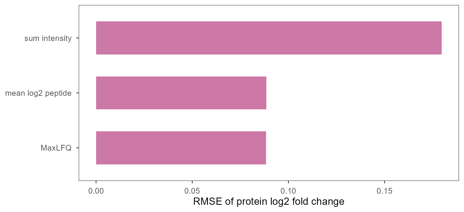
这比”把肽段强度直接相加”稳健,因为中位数比值不会被单个异常肽段带偏;也比”只取一个代表肽段”利用了更多信息。第 33 节的模拟里,MaxLFQ、平均 log2 肽段、直接求和三种做法的 RMSE 分别是 0.088、0.089、0.180;前两者接近,直接求和明显更差。
This is more robust than summing peptide intensities directly, because the median ratio is not dragged by one aberrant peptide, and it uses more information than picking a single representative peptide. In the simulation of Section 33, MaxLFQ, mean log2 peptide and direct summation give RMSEs of 0.088, 0.089 and 0.180; the first two are close and direct summation is clearly worse.
17. iBAQ 与 Top3 / iBAQ and Top3
iBAQ 把蛋白强度除以”理论肽段数”,试图把”蛋白有多长”从”蛋白有多少”里除掉:
iBAQ divides a protein’s intensity by its number of theoretical peptides, trying to remove “how long the protein is” from “how much protein there is”:
\[ \mathrm{iBAQ}_i=\frac{I_i}{n_i^{\text{theoretical}}}. \]
Top3 则取每个蛋白最强的三条肽段,取平均或求和。两者都不是严格的归一化,而是蛋白定量策略:它们决定”一个蛋白的强度”怎么从肽段算出来,之后的样本间归一化仍然要做。把它们与 median/quantile 混为一谈,是蛋白组文献里常见的概念混淆。
Top3 takes the three strongest peptides per protein and averages or sums them. Neither is a strict normalisation; both are protein quantification strategies: they decide how a protein’s intensity is computed from peptides, and sample-level normalisation still has to follow. Treating them as alternatives to median/quantile normalisation is a common conceptual mix-up in proteomics.
本文的 LFQ 数据是肽段级,所以第 33 节能比较 MaxLFQ 与”直接聚合”,但不能比较 iBAQ(缺理论肽段数);这一点在数据与许可一节会再次说明。
The LFQ data here are peptide-level, so Section 33 can compare MaxLFQ with direct aggregation but not iBAQ (theoretical peptide counts are unavailable); Section 23 returns to this limitation.
18. ComBat:批次模型不是归一化 / ComBat: batch models are not normalisation
ComBat 假设批次效应是”位置 + 尺度”的:
ComBat assumes batch effects are “location plus scale”:
\[ y_{ijg}=\alpha_g+X_i\beta_g+\gamma_{bg}+\delta_{bg}\varepsilon_{ijg}, \]
其中 \(g\) 是特征,\(b\) 是批次,\(\gamma\) 与 \(\delta\) 用经验贝叶斯在特征之间收缩。它能把批次差异压掉,但它校正的是批次,不是深度;把 ComBat 当归一化用,会在批次与生物条件不完全平衡时把条件效应一起减掉。
where \(g\) is a feature, \(b\) a batch, and \(\gamma,\delta\) are shrunk across features by empirical Bayes. It removes batch differences, but it corrects batch, not depth; using ComBat as a normaliser can subtract the condition effect when batch and condition are not perfectly balanced.
第 33 节的真实 LFQ 数据里,原始 log2 强度的第一主成分与批次的 \(R^2\) 是 0.048,中位数归一化后降到 0.012,quantile 后是 0.011。中位数归一化顺手压掉了一部分批次,但这是”碰巧”,不是模型;要处理批次,应该显式建模,并检查批次与条件是否可分离。
On the real LFQ data of Section 33, the first principal component of raw log2 intensities has $R^2=0.048 with batch; after median normalisation it falls to 0.012, and after quantile to 0.011. Median normalisation incidentally removes some batch, but that is luck, not a model; to handle batch, model it explicitly and check that batch and condition are separable.
19. scran:池化 size factor / scran: pooled size factors
单细胞的麻烦是”每个细胞测到的基因太少,逐细胞估 size factor 噪声太大”。scran 的办法是把细胞分成若干池,把同一池的计数相加,得到”池的 size factor”,再解一个线性系统,把池因子分解回每个细胞:
Single-cell data have too few counts per cell for a stable per-cell size factor. scran pools cells, sums counts within each pool to get a pool size factor, then solves a linear system to deconvolve pool factors back to individual cells:
\[ \mathrm{sf}_c=\sum_{p}w_{cp}\,\mathrm{sf}_p, \qquad w_{cp}=\frac{\text{counts of cell }c\text{ in pool }p}{\text{total counts of pool }p}. \]
它假设”池内的细胞在组成上大致相同”,因此池化不会把细胞类型差异误当成深度。第 30 节的 PBMC 数据上,scran 因子与文库大小的相关系数是 0.930;在已知细胞类型的模拟里,CPM、scran、sctransform 的 ARI 分别是 0.960、0.995、1.000。三者都接近 1,说明在这个模拟里深度是主要噪声;scran 的优势要在更极端的数据上才明显。
It assumes “cells within a pool have roughly the same composition”, so pooling does not mistake cell-type differences for depth. On the PBMC data of Section 30, the correlation between scran factors and library size is 0.930; in the simulation with known cell types, CPM, scran and sctransform achieve ARIs of 0.960, 0.995 and 1.000. All three are near 1, so depth is the main noise in this simulation; scran’s advantage needs more extreme data to show.
20. sctransform:负二项残差 / sctransform: negative-binomial residuals
sctransform 不做除法,而是为每个基因拟合一个负二项回归,把”测序深度”作为协变量:
sctransform does not divide; it fits a negative-binomial regression per gene with sequencing depth as a covariate:
\[ \log \mu_{cg}=\beta_{0g}+\beta_{1g}\log_{10}\Big(\sum_{g'}x_{cg'}\Big), \qquad z_{cg}=\frac{x_{cg}-\mu_{cg}}{\sqrt{\mu_{cg}+\mu_{cg}^2/\theta_g}}. \]
\(\beta_{1g}\) 与 \(\theta_g\) 在基因之间做正则化收缩,避免低表达基因的拟合爆炸。输出 \(z\) 是”扣掉深度效应后的残差”,可以直接做 PCA 与聚类。
\(\beta_{1g}\) and \(\theta_g\) are shrunk across genes to avoid unstable fits for low-expression genes. The output \(z\) is a residual after removing depth, ready for PCA and clustering.
第 30 节里,sctransform 在模拟数据上的 ARI 是 1.000,在真实 PBMC 上与 scran 的聚类一致性是 0.978,而与 CPM 只有 0.760。这说明它确实改变了细胞之间的距离结构;改变是不是”更好”,需要下游标签才能判断,本文没有真实标签,所以只报一致性,不排优劣。
In Section 30, sctransform reaches an ARI of 1.000 on simulated data; on real PBMC its clustering agreement with scran is 0.978, and with CPM only 0.760. It clearly changes the distance structure; whether the change is “better” needs downstream labels, which the real data lack, so only agreement is reported, not a ranking.
21. CLR 与 ILR / CLR and ILR
CLR 不估计样本因子,而是把每个样本的向量投影到”和为零”的子空间:
CLR does not estimate a sample factor; it projects each sample’s vector onto the sum-zero subspace:
\[ \mathrm{clr}(x)_i=\log x_i-\frac1D\sum_{j=1}^{D}\log x_j . \]
它的输出满足 \(\sum_i \mathrm{clr}(x)_i=0\),因此消除了”总量”这个自由度,也消除了组成约束带来的伪相关。ILR 进一步用正交基把 \(D\) 维降到 \(D-1\) 维,适合直接作为回归的输入。第 31 节的代谢组数据里,raw 与 CLR 的性别 \(R^2\) 分别是 0.129 与 0.129,年龄相关分别是 0.124 与 0.124;在这批已经清理过的数据上,CLR 没有带来可见改善。
Its output satisfies \(\sum_i \mathrm{clr}(x)_i=0\), removing the “total” degree of freedom and the spurious correlations induced by the composition constraint. ILR further reduces \(D\) parts to \(D-1\) orthonormal coordinates suitable for regression. On the metabolomics data of Section 31, raw and CLR give gender \(R^2\) of 0.129 and 0.129, and age correlations of 0.124 and 0.124; on this already clean dataset, CLR brings no visible improvement.
22. Spike-in:唯一能看见全局变化的锚 / Spike-in: the only anchor that sees a global shift
Spike-in 归一化不猜”总量相同”或”多数不变”,而是加入一组已知量的外源分子(ERCC、UPS1 等),用它们的读数估计每个样本的回收率:
Spike-in normalisation does not guess “equal total” or “most unchanged”; it adds a set of known external molecules (ERCC, UPS1, etc.) and uses their reads to estimate each sample’s recovery:
\[ s_j=\frac{\text{spike reads}_j}{\operatorname{median}_k(\text{spike reads}_k)}. \]
这是唯一能在”所有内源基因同时上调”时仍给出正确结论的方法,因为锚点的量不随生物条件变化。第 34 节的模拟里,真实的全局位移是 0.5;SpikeIn 估计出 0.548,而 CPM、TPM、UQ、MoR、RLE、TMM、QN 分别给出 0.067、0.098、0.026、0.023、0.022、0.010、0.013,全部接近 0。
This is the only method that can still be right when every endogenous gene goes up, because the anchor does not change with biology. In the simulation of Section 34 the true global shift is 0.5; SpikeIn estimates 0.548, while CPM, TPM, UQ, MoR, RLE, TMM and QN give 0.067, 0.098, 0.026, 0.023, 0.022, 0.010 and 0.013, all near 0.
代价是锚点本身可能丢失、降解或被基质效应影响;一旦 spike-in 的回收率与内源分子不同,归一化就会引入新的偏倚。所以它也不是”免费的真值”,只是把假设从”内源”换成了”外源”。
The price is that the anchor itself can be lost, degraded or affected by matrix effects; if spike recovery differs from endogenous recovery, normalisation introduces a new bias. It is not free ground truth, only a different assumption: external instead of internal.
23. 四套真实数据与许可 / Four real datasets and their licences
本文用四套真实数据。airway 是 DESeq2 论文附带的 RNA-seq 数据:8 个样本、63,677 个基因、4 个细胞系、地塞米松处理与对照配对;零的比例是 61.1%,文库大小从 15.16 到 30.82 百万。LFQ 稀释系列来自 NormalyzerDE 的示例数据:100 个肽段、27 次运行、9 个浓度各 3 次重复、2 个批次,约 8% 缺失,58 个肽段在 27 次运行中完整。
Four real datasets are used. airway is the RNA-seq data shipped with the DESeq2 paper: 8 samples, 63,677 genes, 4 cell lines, dexamethasone-treated and control paired; the zero fraction is 61.1% and library sizes run from 15.16 to 30.82 million. The LFQ dilution series comes from NormalyzerDE’s example data: 100 peptides, 27 runs, nine concentrations in triplicate, two batches, about 8% missing, with 58 peptides complete across all 27 runs.
| 数据 / Dataset | 规模 / Size | 缺失或零 / Missing or zero | 用途 / Use |
|---|---|---|---|
| airway | 63677 × 8 | 61.1% zeros | bulk DE, depth |
| LFQ dilution | 100 × 27 | ~8% missing | proteomics, batch |
| PBMC 3k | 11139 × 600 | 92.5% zeros | single cell |
| CLL | 409600 × 24 | 0 missing | microarray |
| sacurine | 109 × 183 | 0 missing | metabolomics |
English: one row per dataset; size is features × samples.
PBMC 3k 是 10x Genomics 的公开数据;本文取 600 个细胞、11,139 个基因,零的比例 92.5%。CLL 是 Bioconductor CLL 包的芯片数据(409,600 个探针 × 24 个样本);sacurine 是 ropls 包的尿液代谢组数据(109 个代谢物 × 183 个样本,附年龄、BMI、性别)。四套数据都随包分发,或来自公开数据门户;本文不做任何再分发,只引用包名与链接。
PBMC 3k is public 10x Genomics data; 600 cells and 11,139 genes are used here, with a zero fraction of 92.5%. CLL is the microarray data in the Bioconductor CLL package (409,600 probes × 24 samples); sacurine is the urine metabolomics data in ropls (109 metabolites × 183 samples, with age, BMI and gender). All four are distributed with their packages or come from public portals; nothing is redistributed here, only package names and links are given.
24. 模拟器:把假设写进生成过程 / A simulator that encodes the assumptions
要判断”哪种归一化更好”,必须有真值。本文的模拟器分四层。计数:负二项,均值由基线丰度、样本深度因子、真实 log2 fold change 与长度偏倚相乘;可以控制差异基因比例、方向(平衡/全上调)、全局位移。蛋白组:对数正态强度 + 样本加载因子 + 真实差异 + MNAR 缺失,缺失概率随丰度下降而上升。肽段:每个蛋白 4 条肽段,肽段效应独立,缺失独立于丰度。单细胞:3 个细胞类型,每类 60 个标记基因,细胞特异性 size factor。代谢组:对数正态浓度 + 稀释因子 + 差异。
Judging “which normalisation is better” requires ground truth. The simulator has four layers. Counts: negative binomial, with the mean given by baseline abundance, a sample depth factor, a true log2 fold change and a length bias; the DE fraction, direction (balanced or all-up) and global shift are controllable. Proteomics: log-normal intensities plus sample loading, true effects and MNAR missingness whose probability rises as abundance falls. Peptides: four peptides per protein with independent peptide effects and abundance-independent missingness. Single cell: three cell types, 60 marker genes each, cell-specific size factors. Metabolomics: log-normal concentrations plus a dilution factor and true effects.
这个设计的好处是每个实验只违反一条假设:深度实验只动深度因子,组成实验只动差异比例与方向,长度实验只动长度偏倚,全局实验只动 \(+0.5\) 的全局位移。坏处是它比真实数据干净得多;第 23 节的真实数据用来补上”真实分布”这一块,模拟用来补上”真值”这一块,两者不能互相替代。
The advantage is that each experiment violates one assumption only: the depth experiment moves the depth factor, the composition experiment moves the DE fraction and direction, the length experiment moves the length bias, and the global experiment adds a \(+0.5\) shift to everything. The disadvantage is that it is much cleaner than real data; the real datasets of Section 23 supply “real distributions” and the simulator supplies “ground truth”, and neither replaces the other.
25. E01:真实数据长什么样 / E01: what the real data look like
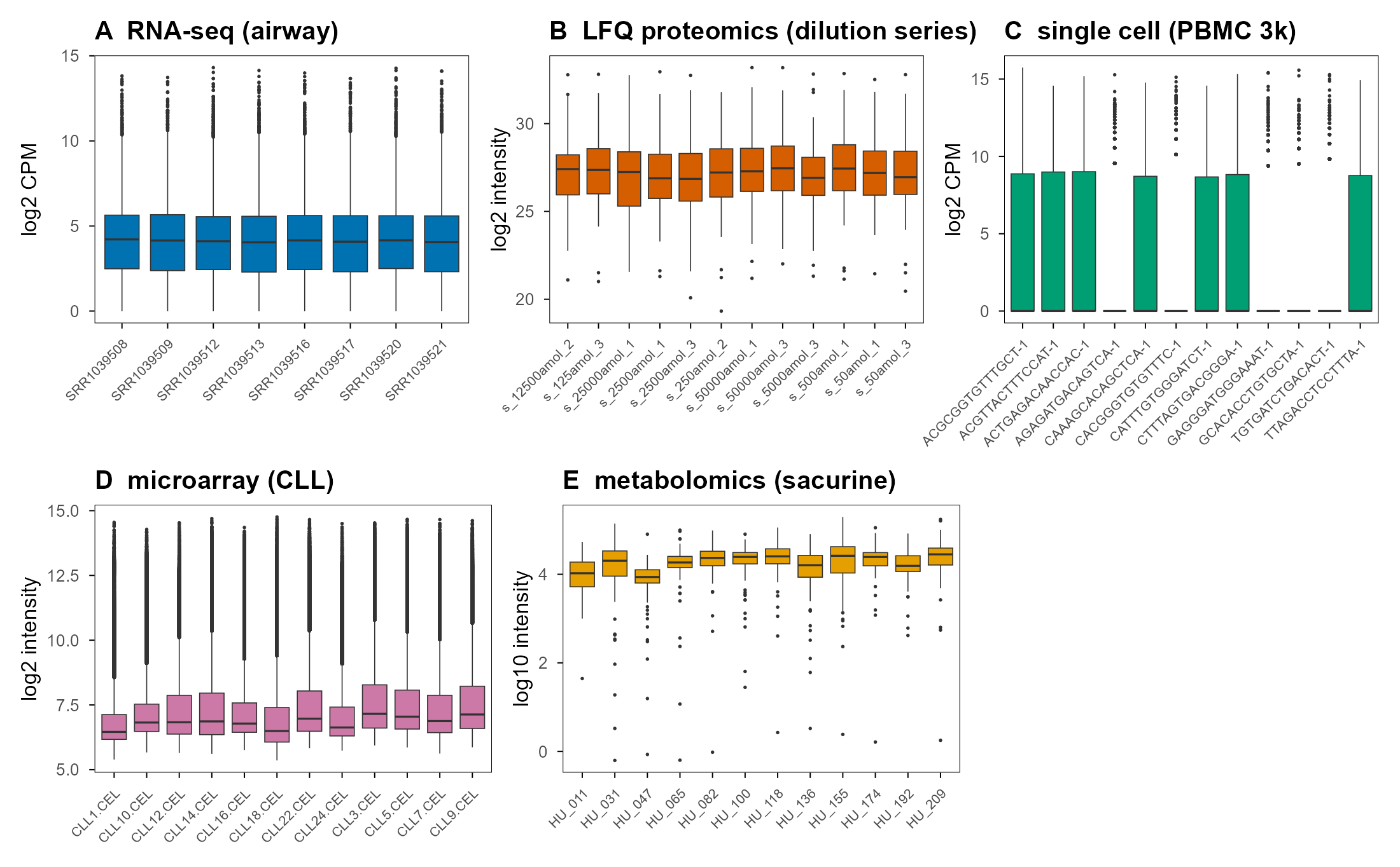
第一组实验不做归一化,只看原始数据的形状。四套数据的量纲、稀疏度与样本结构完全不同:airway 的零比例 61.1%,文库大小相差约 2 倍;LFQ 是 100 个肽段 × 27 次运行,中位样本相关 0.937;PBMC 的零比例 92.5%,绝大多数基因在大多数细胞里没有读数;CLL 是 409,600 个探针 × 24 个样本;sacurine 是 109 个代谢物 × 183 个样本。
The first experiment does no normalisation and only looks at raw shapes. The four datasets differ completely in scale, sparsity and sample structure: airway has a zero fraction of 61.1% and a twofold range of library sizes; the LFQ data are 100 peptides × 27 runs with a median sample correlation of 0.937; PBMC has a zero fraction of 92.5%, with most genes unobserved in most cells; CLL is 409,600 probes × 24 samples; sacurine is 109 metabolites × 183 samples.
airway 的主成分结构值得单独看。第一主成分与处理的 \(R^2\) 在 CPM 下是 0.946,在 UQ 下是 0.908;与深度的相关在 CPM 下是 0.214,UQ 下是 0.341。换句话说,在这批数据上,归一化方法主要改变”深度残留”这一项,几乎没有改变”处理效应”这一项;生物信号太强,方法之间的差异被它盖住了。
The principal-component structure of airway deserves a separate look. The first PC has \(R^2\) with treatment of 0.946 under CPM and 0.908 under UQ; its correlation with depth is 0.214 under CPM and 0.341 under UQ. In other words, on this dataset normalisation mainly changes the residual depth term and barely touches the treatment effect; the biological signal is strong enough to hide the differences between methods.
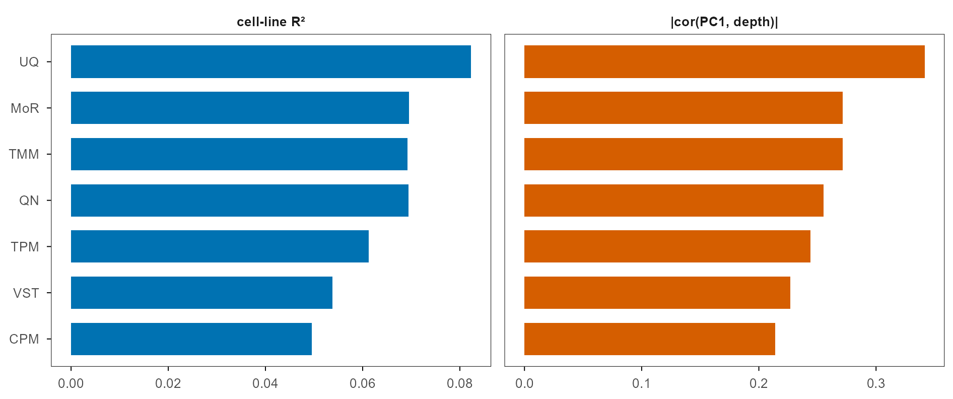
这张图也解释了为什么”只看分布”不够。七种方法的分布都能画得整整齐齐,但深度残留相差 60%。分布图回答”看起来像不像”,主成分回答”还剩下什么结构”。
This figure also explains why “just look at the distributions” is insufficient. All seven methods can be drawn tidy, yet their residual depth differs by 60%. A distribution plot answers “does it look right”; a PCA answers “what structure is left”.
26. E02:只加深度差异 / E02: depth only
第二组只制造深度差异:12 个样本的深度因子取对数正态,标准差 0.6,差异基因 10%,长度与组成都保持中性。五种重复,七种方法。结果在预料之中,也在预料之外。
The second experiment creates depth differences only: log-normal depth factors with standard deviation 0.6 across 12 samples, 10% DE genes, neutral length and composition. Five replicates, seven methods. The result is both expected and not.
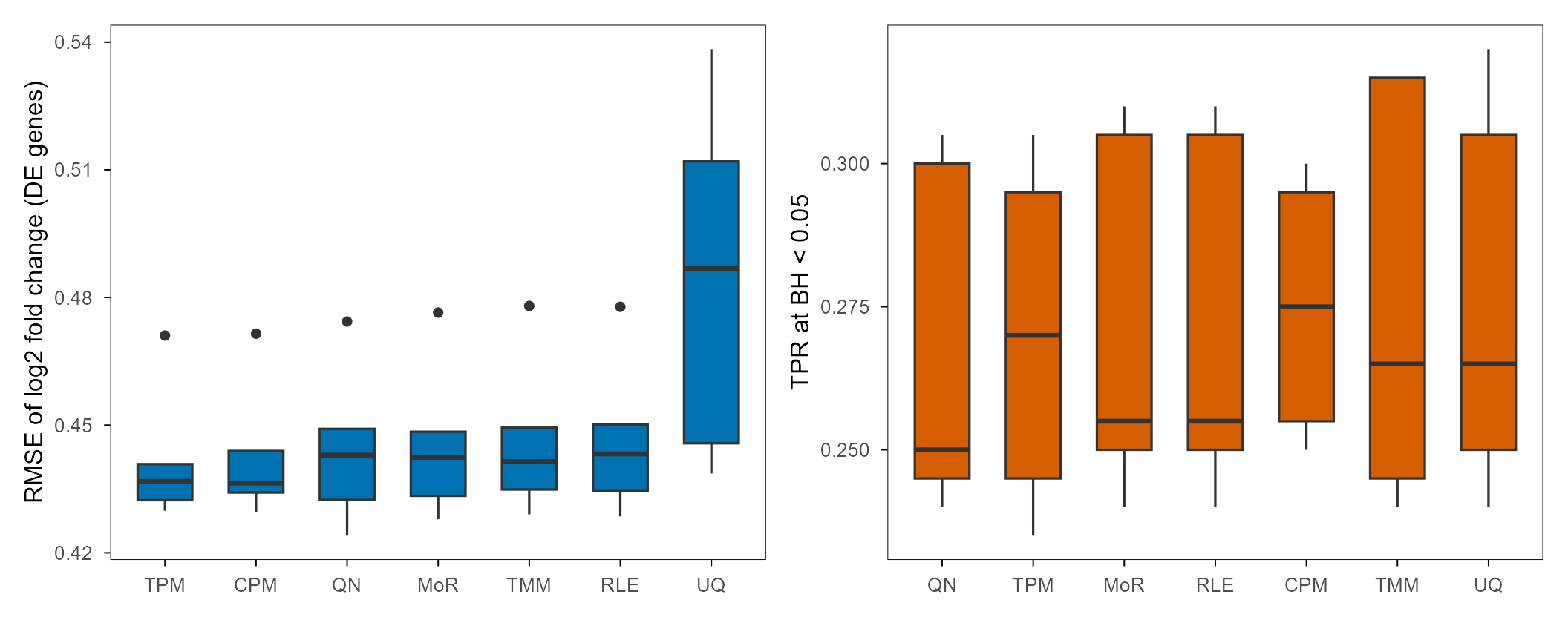
预料之中的是:深度是最好处理的噪声。 CPM、TPM、MoR、RLE、TMM、QN 的 RMSE 都在 0.442–0.484,TPR 都在 0.268–0.276,FDR 在 0.071–0.084。在只有深度差异时,选哪个方法都能得到接近的结论。
What is expected: depth is the easiest noise to handle. CPM, TPM, MoR, RLE, TMM and QN all have RMSE between 0.442 and 0.484, TPR between 0.268 and 0.276, and FDR between 0.071 and 0.084. With depth as the only nuisance, any of these methods gives a similar answer.
预料之外的是 UQ。它的 RMSE 是 0.484,比 CPM 高约 0.041。原因不是 UQ 的假设错,而是估计不稳:11% 的零让 75 分位数落在很稀疏的区域,样本深度一变,分位数就跳到另一个基因上。这提醒我们:一个正确的统计量,如果估计方差太大,也会变成坏方法。
What is unexpected is UQ. Its RMSE is 0.484, about 0.041 above CPM. The assumption is not wrong; the estimate is unstable: with 11% zeros the 75th percentile sits in a sparse region, and a small change in depth moves it to a different gene. The lesson: a correct statistic with high estimation variance is still a bad method.
27. E03:当多数基因都变化 / E03: when most genes change
第三组把差异基因比例从 5% 推到 50%,并且让所有差异都朝同一个方向(全上调)。这直接打击”多数基因不变”的假设。结果是渐进的,不是二元的:偏倚随比例上升,所有方法都向下偏,只是速度不同。
The third experiment pushes the DE fraction from 5% to 50% and makes every effect point the same way (all up). This attacks the “most genes are unchanged” assumption directly. The result is gradual, not binary: bias grows with the fraction, every method drifts downward, only the speed differs.
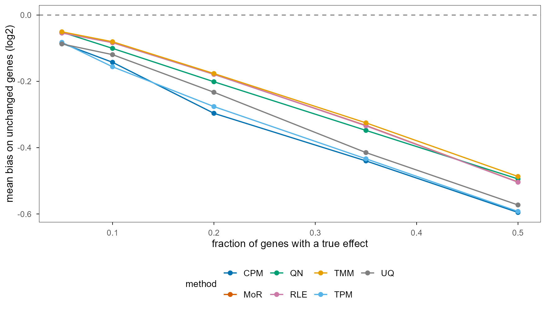
在 50% 处,未变化基因的偏倚分别是:CPM -0.595、TPM -0.592、UQ -0.573、MoR -0.504、RLE -0.504、TMM -0.487、QN -0.494。没有一种方法能把”50% 基因同向上调”与”总量没变”区分开;它们只能把偏倚从 0.60 降到 0.49。
At 50% the bias on unchanged genes is CPM -0.595, TPM -0.592, UQ -0.573, MoR -0.504, RLE -0.504, TMM -0.487 and QN -0.494. No method can distinguish a same-direction shift in 50% of genes from “the total did not change”; they only reduce the bias from 0.60 to 0.49.
这也说明了”多数不变”不是一条安全线。10% 差异时 TMM 的偏倚只有 -0.081,看起来无害;30% 时已经到 。假设不是”成立/不成立”,而是”偏离多少”;报结果时应该报这个连续量,而不是一句”方法对组成变化稳健”。
This also shows that “most unchanged” is not a safety line. At 10% DE, TMM’s bias is only -0.081, apparently harmless; at 30% it is already . Assumptions are not true or false but more or less violated; report the continuous quantity instead of saying “the method is robust to composition”.
28. E04:长度偏倚 / E04: length bias
第四组让计数与基因长度相关:\(\mu_{ij}\propto(\ell_i/\bar\ell)^{0.6}\)。然后比较 CPM 与 TPM 的平均表达与长度的相关。CPM 的相关是 0.184,TPM 是 -0.145——长度校正把正相关翻成了轻微负相关。
The fourth experiment makes counts depend on gene length, \(\mu_{ij}\propto(\ell_i/\bar\ell)^{0.6}\), then compares the correlation between mean expression and length for CPM and TPM. CPM gives 0.184, TPM -0.145 — length correction flips a positive correlation into a slightly negative one.
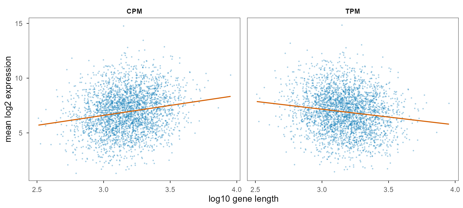
负相关不一定是”校正过头”,也可能是长度与真实表达在这个模拟里负相关(长基因表达更低)。关键是校正后相关从 0.18 变成 −0.15,量级都小;这是因为本文的长度偏倚指数只有 0.6,真实测序的偏倚可能更强。要判断一个数据集需不需要长度校正,最直接的办法是画这张图;如果相关接近 0,TPM 与 CPM 的差异就只是”总量定义”的差异。
A negative correlation is not necessarily “over-correction”; length and true expression may be negatively correlated in the simulation (longer genes expressed lower). The point is that the correlation moves from 0.18 to −0.15, both small, because the length-bias exponent here is only 0.6; real sequencing can be stronger. The direct way to decide whether a dataset needs length correction is to draw this plot; if the correlation is near 0, TPM and CPM differ only in what “total” means.
29. E05:蛋白组的缺失与插补 / E05: missing values and imputation
第五组模拟 1500 个蛋白 × 12 个样本,25% 缺失,缺失概率随丰度下降(MNAR)。四个策略:完整蛋白上的中位数归一化、先做最小插补再做中位数、先做最小插补再做 quantile、完整蛋白上的 VSN。
The fifth experiment simulates 1500 proteins × 12 samples with 25% missing, and missingness rises as abundance falls (MNAR). Four strategies: median on complete proteins, minimum imputation then median, minimum imputation then quantile, and VSN on complete proteins.
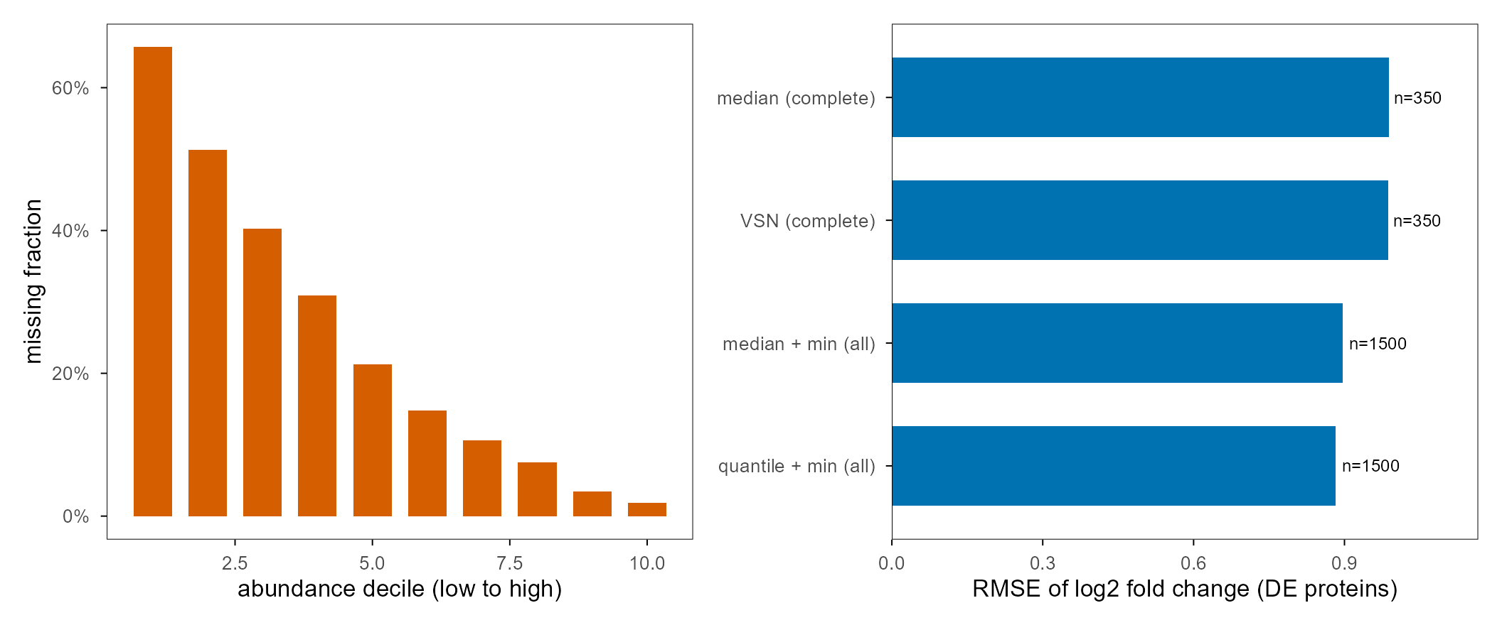
完整蛋白只有 23.3%(350/1500),但它们的 TPR 是 0.943,RMSE 是 0.988。先插补再中位数保留了 1500 个蛋白,RMSE 略降到 0.897,但 TPR 变成 0.000;quantile + 插补的 TPR 也只有 0.040。
Complete proteins are only 23.3% (350/1500), but their TPR is 0.943 and their RMSE is 0.988. Imputation before median keeps all 1500 proteins, lowers RMSE slightly to 0.897, but TPR becomes 0.000; quantile plus imputation reaches only 0.040.
这是全文最刺眼的一组数字。插补不是”保留信息”,而是”制造方差”:把 25% 的值塞到分布最左端,组内方差被抬高,t 统计量被压低,差异蛋白全部消失。RMSE 反而下降,因为插补值靠近 0,把极端估计拉回中间——这正是”指标对了、结论错了”的典型。稳健的做法是先过滤、后归一化,并在正文里报告过滤掉了多少。
This is the most striking set of numbers in the article. Imputation is not “keeping information” but “manufacturing variance”: 25% of values are pushed to the far left tail, within-group variance rises, t-statistics shrink, and every DE protein disappears. RMSE falls because the imputed values sit near 0 and pull extreme estimates toward the middle — a textbook case of “right metric, wrong conclusion”. The robust route is filter first, normalise second, and report how much was filtered.
30. E06:单细胞的三种尺度 / E06: three scales for single cells
第六组用 400 个 PBMC 细胞(1500 个高变基因)与一个已知细胞类型的模拟(600 个细胞 × 1200 个基因,3 类)。比较 CPM、scran 池化因子、sctransform 残差。
The sixth experiment uses 400 PBMC cells (1500 variable genes) and a simulation with known cell types (600 cells × 1200 genes, 3 types), comparing CPM, scran pooled factors and sctransform residuals.
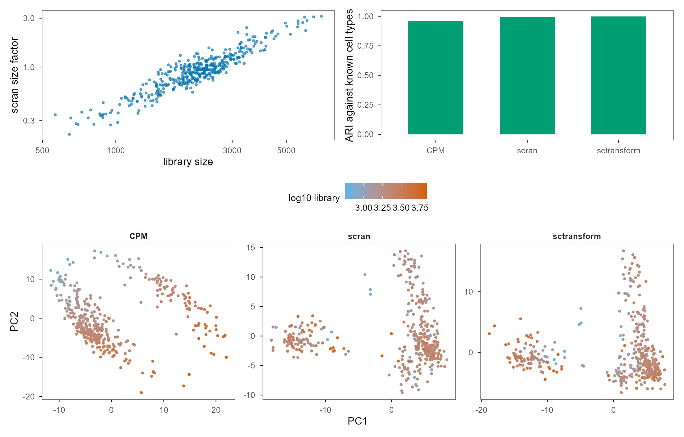
模拟数据上,CPM、scran、sctransform 的 ARI 分别是 0.960、0.995、1.000,都接近 1。真实 PBMC 没有标签,只能看一致性:CPM 与 scran 的 ARI 是 0.760,CPM 与 sctransform 是 0.749,scran 与 sctransform 是 0.978。scran 与 sctransform 高度一致,CPM 与它们分歧明显;这不是谁对谁错,而是”是否把深度当成要移除的结构”。
On simulated data, CPM, scran and sctransform achieve ARIs of 0.960, 0.995 and 1.000, all near 1. Real PBMC has no labels, so only agreement can be measured: CPM versus scran 0.760, CPM versus sctransform 0.749, scran versus sctransform 0.978. scran and sctransform agree closely; CPM disagrees with both — not a matter of right or wrong, but of whether depth is treated as structure to remove.
这里有一个实现上的教训:如果对 scran 归一化后的值再做一次中位数中心化,模拟数据的 ARI 会从 0.995 掉到 0.36。原因是中位数中心化把”每个细胞的组成差异”当成深度差减掉了。单细胞不需要”再归一化一次”;多一步不是更稳,而是把生物信号当噪声。
There is an implementation lesson here: adding median centring on top of scran normalisation drops the simulated ARI from 0.995 to 0.36, because median centring subtracts each cell’s compositional difference as if it were depth. Single cells do not need a second normalisation; the extra step is not more robust, it treats biology as noise.
31. E07:芯片与代谢组 / E07: microarray and metabolomics
第七组用 CLL 芯片(取方差最大的 3000 个探针)与 sacurine 代谢组。芯片比较 raw、quantile、VSN、cyclic loess;代谢组比较 raw、median、quantile、Pareto、CLR。
The seventh experiment uses CLL microarrays (the 3000 most variable probes) and sacurine metabolomics. For arrays it compares raw, quantile, VSN and cyclic loess; for metabolomics raw, median, quantile, Pareto and CLR.
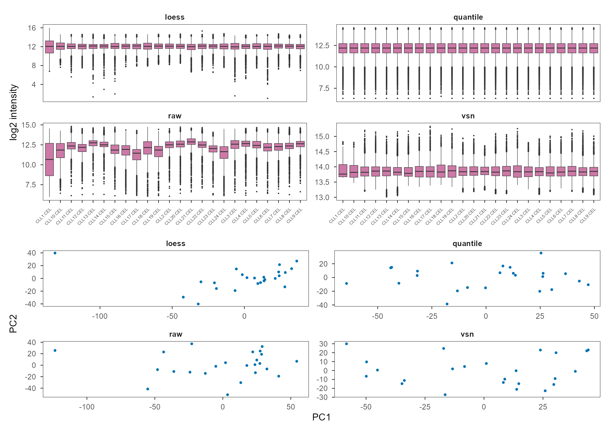
样本间相关的中位数是:raw 0.656、quantile 0.655、VSN 0.701、loess 0.695。quantile 的相关最高,但它的 PCA 曲线最可疑:把分布压成同一条,会把样本间的非线性差异变成一条曲线。这正是”相关性高不等于结构对”的例子。
Median between-sample correlations are raw 0.656, quantile 0.655, VSN 0.701 and loess 0.695. Quantile has the highest correlation but the most suspicious PCA curve: forcing distributions onto one shape turns non-linear differences between samples into a curve. This is “high correlation does not mean correct structure”.
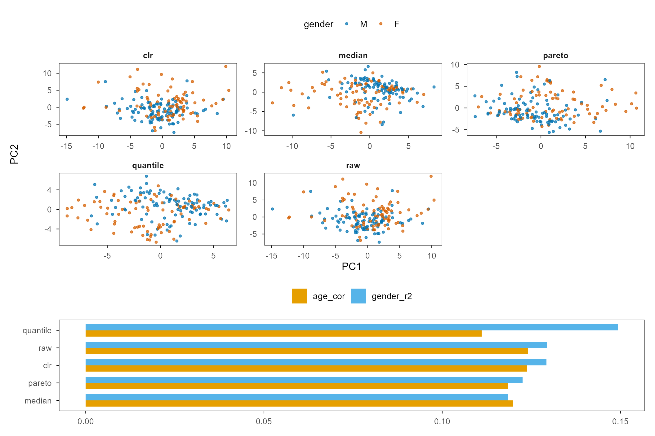
代谢组的结果几乎是”没有差别”。原因是这批数据已经过清理,稀释效应很小;Pareto 与 CLR 主要改变尺度,不改变秩。当归一化不改变秩时,下游的相关系数、PCA 结构、甚至聚类都会几乎不变;这时候选方法的依据不是”效果”,而是”可解释性”与”与已有流程的兼容性”。
The metabolomics result is almost “no difference”. The data are already clean and dilution is small; Pareto and CLR mostly change scale, not ranks. When normalisation does not change ranks, downstream correlations, PCA structure and even clustering barely move; the choice of method is then about interpretability and compatibility with the existing pipeline, not effect size.
32. E08:下游的差异基因集合 / E08: the downstream DE sets
第八组用 airway 的真实处理效应,跑七种归一化 + VST,取 BH < 0.05 且 |log2FC| > 1 的基因集合,算两两 Jaccard。差异基因数量从 TPM 的 134 到 RLE 的 239,Jaccard 从 0.393 到 1。
The eighth experiment uses the real treatment effect in airway, runs seven normalisations plus VST, takes genes with BH < 0.05 and |log2FC| > 1, and computes pairwise Jaccard. DE counts range from 134 with TPM to 239 with RLE, and Jaccard from 0.393 to 1.
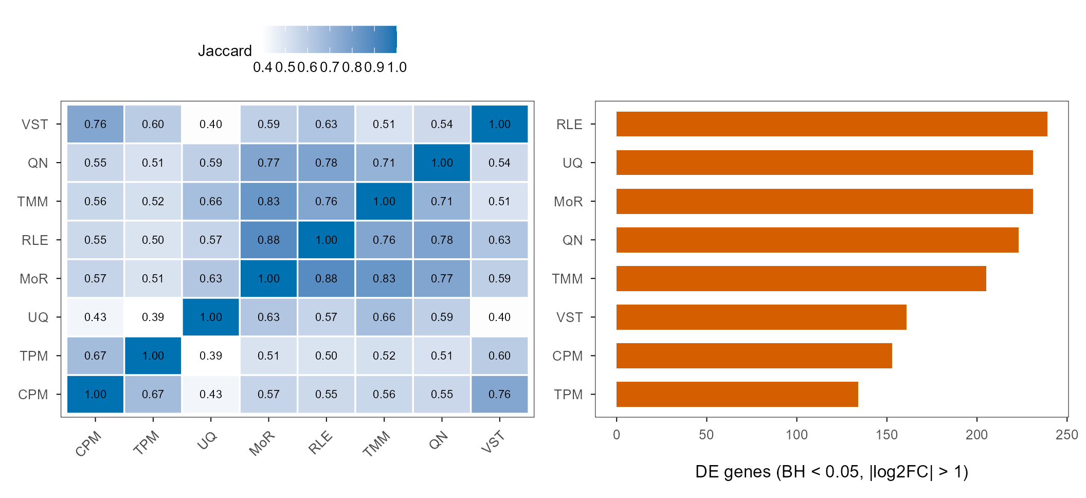
最值得注意的不是”谁最多”,而是 CPM 与 MoR 的 Jaccard 只有 0.567:同一批数据、同一个 limma 流程,仅因为归一化不同,差异基因集合就换掉了约三分之一。归一化不是”预处理”,它会改变你报告的那张表。
What matters is not “which has the most” but that CPM and MoR share only 0.567 of their DE genes: same data, same limma pipeline, a different normalisation changes about a third of the reported list. Normalisation is not preprocessing; it changes the table you publish.
33. E09:两级归一化 / E09: two-level normalisation
第九组看蛋白组的”肽段 → 蛋白 → 样本”两级结构。真实 LFQ 数据上比较 raw、median、quantile、VSN 的组内标准差与批次 \(R^2\);模拟肽段上比较 MaxLFQ、平均 log2 肽段、直接求和。
The ninth experiment looks at the two-level “peptide → protein → sample” structure in proteomics. On the real LFQ data it compares within-group SD and batch \(R^2\) for raw, median, quantile and VSN; on simulated peptides it compares MaxLFQ, mean log2 peptide and direct summation.
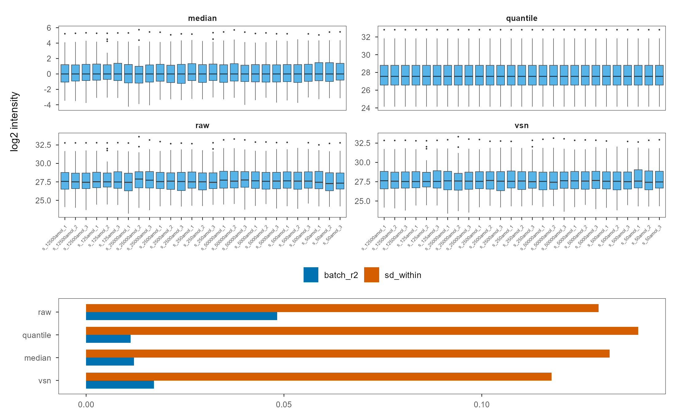
真实数据的组内标准差在四种处理间几乎不变(0.118–0.140),批次 \(R^2\) 却从 0.048 降到 0.011。归一化主要改变样本间的关系,不改变技术重复的精度;这符合预期,但也提醒我们:用”组内 CV 降低”来证明归一化有效,可能什么也证明不了。
Within-group SD barely moves across the four treatments (0.118–0.140), while batch \(R^2\) falls from 0.048 to 0.011. Normalisation changes between-sample relations, not technical precision; that is expected, but it warns against “within-group CV went down” as proof that normalisation worked.
34. E10:全局位移,所有组成法的盲点 / E10: the global shift no composition method can see
第十组让所有基因同时上调 0.5(log2),再加入 50 个不随条件变化的 spike-in 特征。真实的全局位移是 0.5;如果没有外部锚点,任何只看比例的方法都看不见它。
The tenth experiment raises every gene by 0.5 (log2) and adds 50 spike-in features that do not change with condition. The true global shift is 0.5; without an external anchor, no method that sees only proportions can detect it.
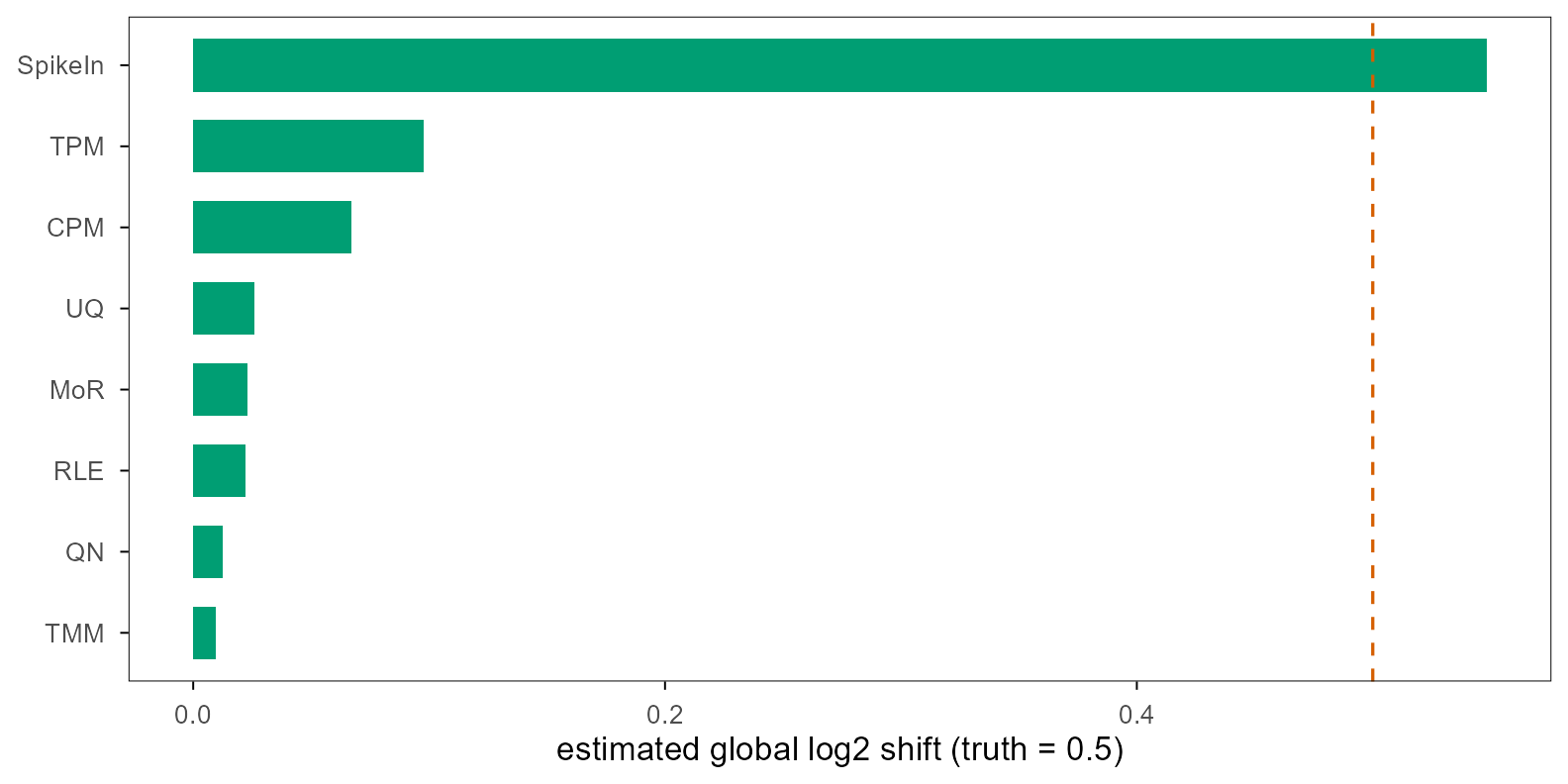
这不是”方法不够好”,而是信息不在数据里。CPM 看到的总量翻倍,会把它解释成”每个基因都没变,只是测序更深”;TMM 与 RLE 看到所有比值不变,会得出同样的结论。只有 spike-in 能说”总量确实翻倍了”。当研究问题涉及全局变化(如整体翻译水平、整体蛋白合成速率),必须设计 spike-in,而不是事后选一个归一化方法。
This is not “the method is not good enough” but the information is not in the data. CPM sees the total double and explains it as “no gene changed, sequencing was deeper”; TMM and RLE see every ratio unchanged and conclude the same. Only spike-ins can say “the total really doubled”. When the question involves global change (global translation, overall protein synthesis), design a spike-in; do not pick a normalisation method afterwards.
35. E11:方法 × 场景总图 / E11: methods × scenarios
最后一组把四种场景放在一起:深度、组成、长度、全局。每种方法在每种场景下算一个 RMSE(对真值),再按场景归一化到 0–1 显示颜色,格子里写原始 RMSE。
The last experiment puts four scenarios together: depth, composition, length and global. Each method gets one RMSE against truth per scenario; colours are min–max scaled within each scenario, and the raw RMSE is printed in each cell.
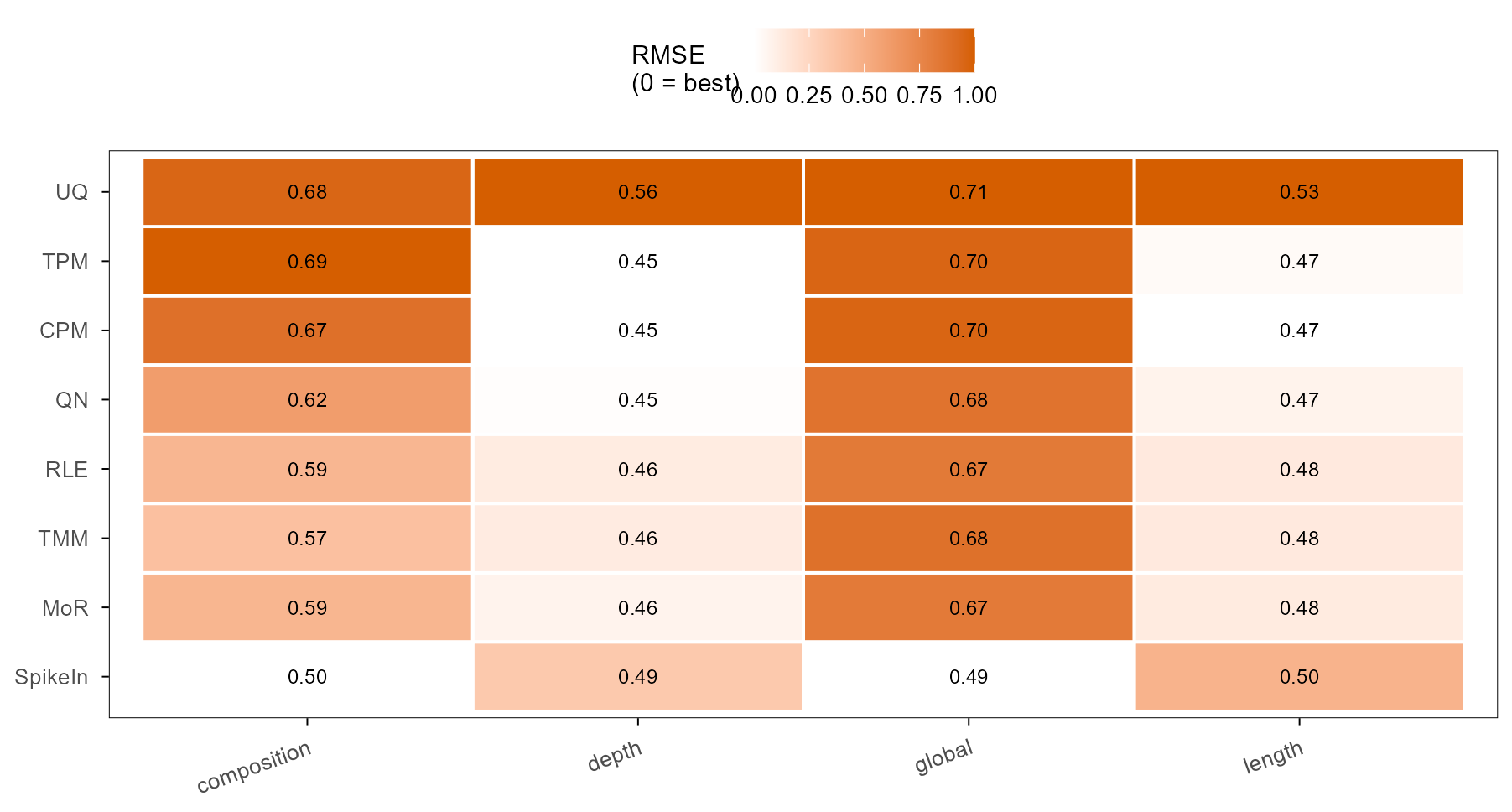
这张图不是”排名”,而是”没有全能选手”。SpikeIn 在三个场景最好,但它的代价是要额外实验;UQ 在深度与长度最差,但在组成场景并不差;CPM/TPM 在深度最好之一,在组成最差。选择归一化方法,本质上是在选择你愿意在哪个场景承担多大的偏差。
This is not a ranking but a demonstration that there is no all-round winner. SpikeIn is best in three scenarios but costs an extra experiment; UQ is worst in depth and length but not bad in composition; CPM/TPM are among the best in depth and the worst in composition. Choosing a normalisation is choosing which scenario you are willing to be biased in.
36. 决策树与十个常见错误 / A decision tree and ten common mistakes
如果把全文压成一张决策树,顺序是:先问有没有 spike-in;再问数据是计数还是强度;再问预期差异是少数还是全局;最后问下游是差异分析还是聚类/降维。 有 spike-in 就用它;计数数据从 CPM/TPM 起步,差异分析优先 MoR/RLE/TMM;强度数据从 median 或 VSN 起步;单细胞用 scran 或 sctransform;需要批次校正时单独建模,不要与归一化混在一起。
Compressed into a decision tree: first ask whether there is a spike-in; then whether the data are counts or intensities; then whether the expected change is sparse or global; finally whether downstream is DE or clustering/dimension reduction. Use the spike-in if present; start counts with CPM/TPM and prefer MoR/RLE/TMM for DE; start intensities with median or VSN; use scran or sctransform for single cells; model batch separately and do not conflate it with normalisation.
十个常见错误,按我见到的频率排序:
Ten common mistakes, ordered by how often I see them:
- 对已经归一化的数据再归一化一次。 比例数据再做中位数中心化,会把真实的组成差异当深度减掉。
Normalising data that are already normalised: median-centring proportions subtracts real composition as if it were depth. - 把 RLE/TMM 因子直接除,不乘文库大小。 因子是相对的,有效文库是 \(\text{lib}\times s\)。
Dividing by RLE/TMM factors without multiplying by library size; the factor is relative and the effective library is \(\text{lib}\times s\). - 用 TPM 做差异分析。 TPM 的总和被强制为 \(10^6\),差异会被组成效应吸收;用 counts 或 logCPM 更合适。
Using TPM for DE: the forced \(10^6\) sum absorbs effects into composition; use counts or logCPM. - 先插补再归一化,或反过来,却不检查顺序的影响。 第 29 节显示顺序可以把 TPR 从 0.94 打到 0。
Imputing before or after normalisation without checking the order; Section 29 shows TPR moving from 0.94 to 0. - 把 ComBat 当归一化。 它校正批次,不校正深度;批次与条件混杂时会减掉生物效应。
Treating ComBat as normalisation: it corrects batch, not depth, and can subtract biology when batch is confounded. - 用 median centring 处理全局变化。 全局变化正是中位数要消掉的东西。
Using median centring for global change, which is exactly what the median removes. - 对稀疏计数做 quantile normalization。 大量并列零让秩序列失去意义,PCA 会出现曲线伪结构。
Quantile-normalising sparse counts: ties at zero make the rank profile meaningless and produce curved PCA artefacts. - 只看分布图或样本相关性。 它们可以很漂亮,同时把差异基因换掉三分之一。
Judging by distribution plots or sample correlation alone: they can look perfect while a third of the DE list changes. - 只报一个指标、一个种子。 RMSE、TPR、FDR、ARI 会给出不同排序;单种子无法区分方法差异与噪声。
Reporting one metric and one seed: RMSE, TPR, FDR and ARI rank methods differently, and a single seed cannot separate method from noise. - 忽略缺失机制。 MNAR 缺失本身携带丰度信息;把它当随机缺失,插补就会系统性地偏。
Ignoring the missingness mechanism: MNAR carries abundance information, and treating it as random biases imputation.
37. 参考文献 / References
- Love, M. I., Huber, W., Anders, S. (2014). Moderated estimation of fold change and dispersion for RNA-seq data with DESeq2. Genome Biology 15, 550. doi:10.1186/s13059-014-0550-8
- Robinson, M. D., McCarthy, D. J., Smyth, G. K. (2010). edgeR: a Bioconductor package for differential expression analysis of digital gene expression data. Bioinformatics 26, 139–140. doi:10.1093/bioinformatics/btp616
- Robinson, M. D., Oshlack, A. (2010). A scaling normalization method for differential expression analysis of RNA-seq data. Genome Biology 11, R25. doi:10.1186/gb-2010-11-3-r25
- Ritchie, M. E., et al. (2015). limma powers differential expression analyses for RNA-sequencing and microarray studies. Nucleic Acids Research 43, e47. doi:10.1093/nar/gkv007
- Huber, W., von Heydebreck, A., Sültmann, H., Poustka, A., Vingron, M. (2002). Variance stabilization applied to microarray data calibration and to the quantification of differential expression. Bioinformatics 18, S96–S104. doi:10.1093/bioinformatics/btg264
- Cox, J., Hein, M. Y., Luber, C. A., Paron, I., Nagaraj, N., Mann, M. (2014). Accurate proteome-wide label-free quantification by delayed normalization and maximal peptide ratio extraction, termed MaxLFQ. Molecular & Cellular Proteomics 13, 2513–2526. doi:10.1074/mcp.M113.031591
- Lun, A. T. L., McCarthy, D. J., Marioni, J. C. (2016). A step-by-step workflow for low-level analysis of single-cell RNA-seq data with Bioconductor. F1000Research 5, 2122. doi:10.12688/f1000research.9501.2
- Hafemeister, C., Satija, R. (2019). Normalization and variance stabilization of single-cell RNA-seq data using regularized negative binomial regression. Genome Biology 20, 296. doi:10.1186/s13059-019-1874-1
- Johnson, W. E., Li, C., Rabinovic, A. (2007). Adjusting batch effects in microarray expression data using empirical Bayes methods. Biostatistics 8, 118–127. doi:10.1093/biostatistics/kxj037
- Willforss, J., Chawade, A., Levander, F. (2019). NormalyzerDE: online tool for improved normalization of omics expression data and high-sensitivity differential expression analysis. Journal of Proteome Research 18, 732–740. doi:10.1021/acs.jproteome.7b00873
- Wagner, G. P., Kin, K., Lynch, V. J. (2012). Measurement of mRNA abundance using RNA-seq data: RPKM measure is inconsistent among samples. Theory in Biosciences 131, 281–285. doi:10.1007/s12064-012-0162-3
- Aitchison, J. (1986). The Statistical Analysis of Compositional Data. Chapman and Hall. (CLR/ILR 的经典来源;书,无 DOI。)
- Bioconductor packages:
airway,CLL,ropls,vsn,limma,edgeR,DESeq2,scran,sctransform,NormalyzerDE. https://bioconductor.org - 10x Genomics PBMC 3k dataset. https://www.10xgenomics.com/datasets
引用说明:第 1–12 条是方法与数据来源,第 13–14 条是软件与公开数据门户。本文的代码、图与
metrics.json在文章目录的R/、scripts/、figures/与outputs/下,可直接重跑。Citation note: items 1–12 are the methods and data sources; items 13–14 are software and public data portals. Code, figures and
metrics.jsonlive underR/,scripts/,figures/andoutputs/in the post directory and can be rerun directly.